
Manufacturing Dive reported on 18 June 2026 that Goodwill South Florida had implemented a Lectra platform at its Miami apparel facility. The underlying vendor announcement concerned cutting-room planning and described expected improvements. This is an attributed deployment announcement, not a published distribution of observed completion times. It provides a starting point for an independent measurement question: what can a duration average reveal, and what does it leave unresolved?
All datasets below are invented examples of ordinary business tasks. They are not measurements from Goodwill, Lectra or an apparel operation. The analysis compares an average with the proportion completed within a chosen duration, the middle observations and the longest observations. These descriptions answer different questions. Keeping them separate helps explain how a lower average can coexist with a longer exceptional completion, without claiming that such a pattern occurred at the reported facility.
An average preserves a sum, not its arrangement
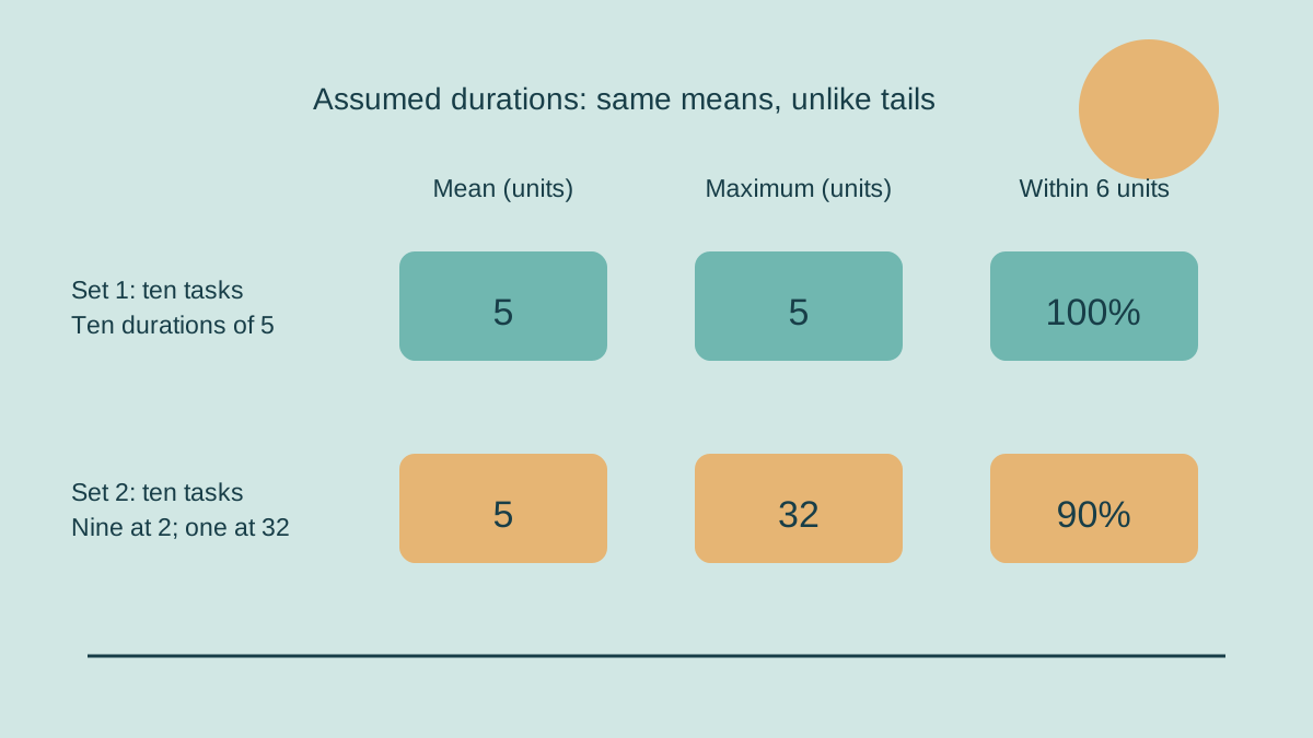
Imagine ten completed tasks, each taking five abstract time units from a defined start to a defined finish. Their durations add to fifty. Dividing by ten gives an arithmetic mean of five. Now imagine a different set containing nine tasks of two units and one task of thirty-two. These durations also add to fifty and produce the same mean of five. The average agrees although the experiences represented by the two sets differ substantially.
The first set has no variation in the invented durations. The second has nine relatively short observations and one much longer observation. The mean does not identify which of these arrangements generated it. It records the sum divided by the observation count. To recover the arrangement, one needs additional information about the individual durations or a description of their distribution. A single accurate average can therefore be insufficient for a question about how often a particular duration is exceeded.
This is not a defect in arithmetic. It is a mismatch between the information preserved by the statistic and the information requested by the question. The mean answers one useful question about the recorded set. It does not promise that every task takes five units, that five is the longest duration or that five is a deadline met by everyone. Each of those statements would add a property that the calculation alone has not established.
A duration threshold asks a different question
Choose a threshold of six abstract time units and count observations completed in six or fewer. The first invented set has ten out of ten, or one hundred per cent, within that threshold. The second has nine out of ten, or ninety per cent. Both means remain five. The threshold comparison reveals a distinction concealed by the averages because it asks how many individual durations satisfy a specified condition rather than how their total is allocated across observations.
The threshold must be stated explicitly, including whether equality counts. In this example, six is included: a task taking exactly six would qualify. Changing the threshold changes the question. At a threshold of one unit, neither set has a qualifying observation. At a threshold of three, the second has nine while the first has none. There is no contradiction. Different thresholds examine different parts of the two invented distributions and need not rank them in the same order.
The count also needs a defined denominator. Here it is the ten completed tasks included in each invented set. It is not all customers, all items produced or all tasks ever started. A proportion based on that denominator describes that set. If another report uses orders while this one uses tasks, the percentages do not automatically represent comparable units. The choice of observation is part of the meaning of the proportion, rather than a detail to add after interpreting it.
A lower mean can coexist with a longer extreme
Consider a third invented set: nine durations of one unit and one duration of twenty. The total is twenty-nine and the mean is two point nine. This mean is lower than the first set’s five. Yet the longest duration is twenty, compared with five in the first set. At the six-unit threshold, the third set still records nine qualifying observations out of ten. The average has improved while these other descriptions have not improved in the same way.
It would be accurate to say that the third set has a lower recorded mean than the first. It would be inaccurate to say that every observation is shorter than every observation in the first. The twenty-unit observation disproves that extension within the invented data. Similarly, a lower mean does not establish a higher proportion within six units. The third set has ninety per cent against the first set’s one hundred, despite its lower mean.
These comparisons do not identify a universally preferable set. A decision might care about total duration, a chosen threshold or exceptional cases, and the example does not assign values to those objectives. The point is to disclose which property supports a particular statement. An average comparison can be valid while being incomplete for a promise about individual completion. The missing information should remain visible rather than being supplied through an attractive but unsupported generalisation.
The middle and the upper end preserve other information
For ten sorted observations, define the median here as the average of the fifth and sixth values. In the first set those values are both five, so the median is five. In the second they are both two, giving a median of two. In the third they are both one, giving a median of one. The median describes the middle of the ordered observations using that stated convention. It does not replace the mean or the longest observation.
One can also define an empirical percentile by a specific rule. Under the nearest-rank rule used here, multiply the observation count by the desired proportion, round upward to the next whole rank and select that sorted observation. For a ninety-fifth percentile and ten observations, the rank is ten. The selected values are therefore five, thirty-two and twenty for the three sets. This small-sample result follows the rule; it is not a forecast of future completion times.
The convention matters because a different interpolation rule can produce a different displayed percentile from the same small set. A report should identify the rule before treating two percentile figures as directly comparable. Stating the rule also prevents an empirical description from being mistaken for evidence that ninety-five per cent of all future tasks will finish within that value. The example contains ten observed fictional durations and supplies no basis for that future-population claim.
Define the clock before comparing its readings
A duration requires a start and a finish. For an invented administrative task, the start could be receipt of a complete request and the finish could be availability of a completed response. Another measure could start at the first incomplete enquiry or finish at delivery to the recipient. These are different boundaries. Even if both measures use hours, their averages would not describe the same interval. A common unit does not make unlike clocks comparable.
The same caution applies to interruptions. One hypothetical record might count elapsed time continuously, while another counts only time spent working on the task. Both can be meaningful with clear definitions. A task with one unit of active work and four units waiting has five units elapsed under the first definition and one unit under the second. The difference comes from the measurement boundary, rather than an inconsistency in the recorded task itself.
A useful comparison therefore names the clock, the observation unit and the inclusion rule before examining the distribution. That preparation does not determine the outcome. It establishes what the outcome means. In the reported deployment, the vendor’s planning boundary should not be silently expanded into an end-to-end apparel completion boundary. The independent examples here make no estimate of either interval; they show why a duration statistic needs its own clearly stated object.
Unfinished tasks are not zero-duration completions
Suppose an invented review begins with ten tasks, of which nine are completed and one remains open at the observation date. If the completed tasks each took two units, their completed-case mean is two. The open task cannot be added as a zero-duration completion to make the mean lower. Its final duration has not been observed. Recording it as zero would invent an outcome, confuse the observation state and change the denominator without acknowledging the change.
If the open task has already elapsed for eight units, its eventual duration is at least eight under the stated continuous clock. That is a lower bound, not a final value. It is already known not to fall within the six-unit threshold, provided its start and the threshold use the same definition. If it has elapsed for only three units, whether it will qualify remains unresolved. The two open observations carry different information even though neither is completed.
This distinction makes a complete statement possible without inventing a finish. A report can say that nine completed durations are known and one task remains open with a stated age. It can separately describe the completed-case mean and the information available about threshold status. The mean of eventual durations for all ten is still unknown. Keeping that unknown prevents a convenient completed-only statistic from being presented as the final result for the entire starting group.
Observation windows can change the apparent sample
A short observation window can include many quick completions while leaving longer tasks unfinished. In an invented starting group, this can make the completed-case distribution look different from the eventual distribution of the whole group. This is a logical consequence of selecting cases by completion before a cutoff. It is not a statement that any real provider excluded difficult cases. The example explains why a completed-only set and a start-defined group should be identified separately.
Comparisons across windows also need a common selection rule. A set of tasks started during one month differs from a set finished during that month. Some tasks finished in the month may have started earlier; some started in the month may finish later. The calendar label alone does not establish which group is included. A distribution headed with a month therefore needs an explanation of whether membership follows start, finish or another defined event.
Neither selection is inherently useless. A finished-case set can describe the completions observed in the period. A start-defined group can support a later account of what happened to that group. The error arises when the first description is treated as the second without checking membership. Defining the group and retaining unresolved cases makes it possible to understand the statistic’s scope without turning missing outcomes into either successes or failures by assumption.
Case mix can change without a change within each class
Imagine two fictional classes of completed tasks. Every task in one class takes two units; every task in the other takes eight. A set containing eight short-class tasks and two long-class tasks totals thirty-two units and has a mean of three point two. Reverse the counts to two short and eight long, and the total becomes sixty-eight with a mean of six point eight. The class-specific durations have not changed, although the combined mean has.
At the six-unit threshold, the first mixture records eighty per cent within the threshold and the second twenty per cent. These percentages accurately describe their invented mixtures. They do not demonstrate that either class became faster or slower. The mix changed. A statement about the overall experience can retain the aggregate comparison, while a statement about performance within a class needs the corresponding class-level observations rather than the combined statistic alone.
This is another reason to preserve several descriptions together. The aggregate distribution describes what the selected group contained. The class composition explains one possible source of its shape. A comparison can show both without pretending that the aggregate should be ignored or that it proves a change inside every class. The hypothetical calculations identify the changing input explicitly, avoiding a causal claim about a software deployment or an employer that the data does not contain.
An exceptional observation needs context, not automatic deletion
The thirty-two-unit observation in the second invented set has a large effect on its mean. That influence does not make the observation invalid. If it meets the stated start, finish and inclusion definitions, removing it changes the set being described. A separate account excluding a defined class can be useful, but it should name that class and disclose the exclusion. Otherwise the reported average may appear to concern all ten observations while actually describing only nine.
A genuine recording error would present a different question. In a fictional record, someone might enter the wrong time unit or attach a finish to the wrong start. Correcting an established error is different from deleting a valid duration because it is inconveniently long. The example offers no real error diagnosis. It separates two reasons for changing a dataset so that an explanation of the revised statistic can identify which reason applies and what evidence supports it.
It can also be informative to show the influence directly. For the second set, the nine two-unit observations total eighteen; the remaining observation contributes thirty-two to the fifty-unit sum. This decomposition explains why the mean is five while most observations are two. It does not declare the longest case unimportant or the shorter cases unrepresentative. It makes the arithmetic visible and leaves any decision about scope attached to an explicit question about the group.
A compact duration report can retain the distinctions
A report does not need to include every individual record in its headline. It does need enough information for the intended claim to be assessed. For the invented ten-task groups, a mean accompanied by the observation count and threshold proportion would already distinguish some properties hidden by the mean alone. Adding the maximum and a clearly defined middle or upper-rank statistic provides other views. The selection should follow the question rather than the desire to display many numbers.
- State the task unit, the start event and the finish event.
- Identify how observations enter the group and its time window.
- Give the count of completed and unresolved observations separately.
- Name the duration threshold and whether equality qualifies.
- Keep the mean, middle, threshold proportion and extreme descriptions distinct.
- Specify any percentile convention and any exclusion or class split.
These fields are an original proposed reporting structure for the fictional examples. They do not describe the systems used at Goodwill or Lectra. Their purpose is to connect each statistic to an inspectable definition. A reader can then distinguish a measured property of the recorded set from an assumption about unfinished cases, a change in composition or an unverified expectation about future tasks.
The central insight is that completion time has a distribution, even when a report displays only one number. An average can fall while a long exceptional observation grows, and equal averages can conceal different threshold proportions. Describing those distinctions makes a timing claim more precise. It also preserves the boundary between a company’s announced expectation and the observations that would be needed to evaluate an actual set of completed tasks.
Sources: Manufacturing Dive, 18 June 2026; Lectra announcement via Business Wire, 16 June 2026. Datasets and statistical examples are original.